Podaris:Insight Street Catchment Analysis

What is Podaris:Insight?

Podaris:Insight is a toolkit for simplifying a number of types of accessibility analysis. It is designed to dramatically speed up the process of performing accessibility analysis on networks and datasets created or imported in Podaris.

It provides a simple interface through which analysis projects can be created and shared, and the corresponding results exported. You can learn more about Podaris:Insight and the analysis types that it offers here.

What is the street catchment analysis type?

The street catchment analysis type measures banded walking or cycling access from a qualifying part of a street network. You can answer questions like:

How much of a city, area-wise, is within 400 m of physically segregated cycle provision?
How many people live within 100 metres of a dedicated walking route?
How many schools are there within 50 metres of a traffic-free paths with no motor vehicles?
What percentage of the entire road network has a pavement?

You choose a Streets project, define which links qualify, and the analysis returns coverage bands on the map, any dataset queries you set, and the area that is not reached.

Unlike stop catchment and isochrone analysis, which measure from points, street catchment measures from a network.

Tip: To measure the benefit of a proposed scheme, build it in the street editor, publish it as a second view, then run this analysis against each view in turn. The difference between the two uncovered figures is the benefit.

Qualifying streets

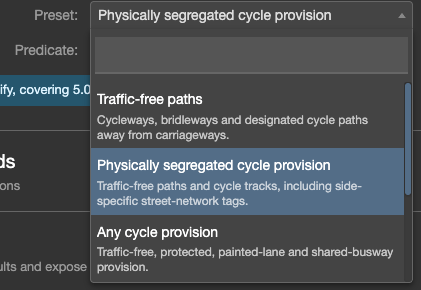
Qualifying streets are the links people need to reach. Choose a preset, or click Edit next to Predicate to build your own rule from street attributes.

Traffic-free paths: cycleways, bridleways and designated cycle paths away from carriageways.
Physically segregated cycle provision: traffic-free paths plus cycle tracks alongside roads, including side-specific provision. This is the default.
Any cycle provision: everything above, plus painted lanes and shared bus lanes.
Dedicated walking routes: footways, pedestrian streets and paths designated for walking.
Streets with pavements: links explicitly recorded as having a pavement.

Each preset also excludes links the chosen mode is banned from, so a cycleway closed to cycles does not count towards cycle provision.

A preview line reports how much of the network your rule matched before you run anything. It is worth reading: a preset that matches almost nothing usually means the attribute is not recorded in your area, not that the provision does not exist.

Caution: The presets read what is recorded in the street network. A street with a cycle track that nobody has tagged will not qualify. If coverage looks wrong, check the preview and inspect a few streets in the street editor.

Step by Step

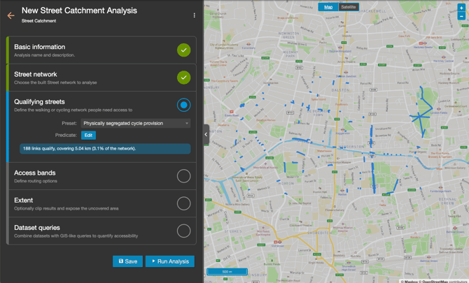
1. Add basic information such as a name and description that will be visible to viewers of the project.

2. Select a street network and a view to analyse. The analysis uses the published network for that view, so unpublished edits made in the street editor are not included. Rebuild the network first if you want your latest changes analysed.

3. Choose the qualifying streets, using a preset or a custom predicate, as described above.

4. Define your access bands. Choose whether to measure by distance or travel time, then set up to ten bands. For distance you can also choose whether to follow the street network or use straight-line distance. Finally choose the mode people travel by to reach the network, walk or cycle. Note this is how people reach the qualifying streets, not what those streets are for: walking access to cycle provision is a normal thing to measure.

5. Set the extent (optional). Draw or import a single boundary polygon to clip the results to your study area. Left empty, the boundary the street network was extracted with is used where one exists. The boundary is what turns coverage into a percentage and produces the uncovered area.

6. Add dataset queries (optional). Connect up to five datasets and query them against the bands, as in any other analysis, to turn a coverage percentage into a population figure. See isochrone queries.

Interpreting results

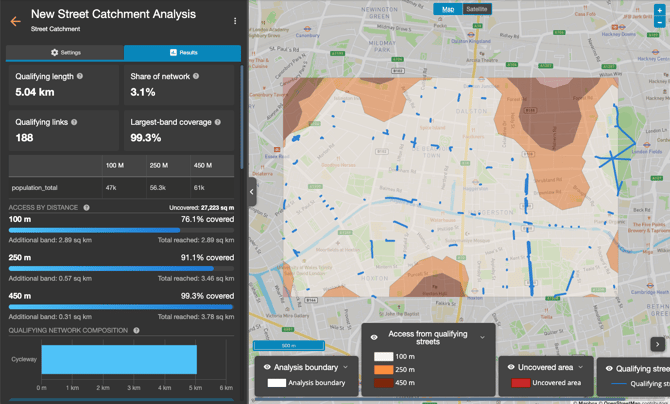
The results page opens with headline figures about the qualifying network itself.

Qualifying length is the total length of matched links, counting parallel carriageways and separately mapped links independently.
Share of network expresses that as a proportion of the whole network in the selected version.
Qualifying links counts the matched links, though length is the better comparison because link boundaries are a mapping artefact.
With a boundary set, largest-band coverage gives the share of it reached within the widest band.

The banded chart below shows what each band adds and what has been reached in total, along with the uncovered area. Bands are non-overlapping rings, so the additional-band figure is new ground, not a running total.

Qualifying network composition breaks the matched length down by street type. Use it as a check on your rule: if you asked for segregated provision and most of the matched length is footways, the rule is catching more than you meant.

Any dataset queries appear as a table across the bands.

Styling the results

Four layers can be styled independently in the display settings: the catchment bands, the qualifying streets, the uncovered area and the boundary.

Exporting results

Your analyses can be exported by clicking the project name, and Export Analyse. Street catchment offers five exports, four spatial and one tabular.

Each of the GIS exports can be downloaded as GeoJSON, Shapefile, KML or CSV, and opens directly in QGIS, ArcGIS and most other GIS software.

Catchment bands (GIS): the access bands as non-overlapping rings. Each polygon is the ground that band adds and nothing more, so the areas can be summed or shaded without double counting. Use this for a banded choropleth.
Cumulative catchments (GIS): the same bands as nested, overlapping polygons, each covering everything reachable within that distance or time. Use this when you want a single "within 400 m" polygon to clip or intersect against other data.
Qualifying streets (GIS): the links the predicate matched, as lines. Useful for showing the network the catchment was measured from, and for checking the rule caught what you intended.
Uncovered area (GIS): the part of the analysis boundary beyond the largest band. This is often the output that carries a business case, since it is the gap a scheme would close.
Street Catchment summary (CSV): one row per band, with the distance or travel time, the band area, the cumulative area, and a column for each dataset query you set up. This is the table to paste into a report or a spreadsheet model.