Isochrone queries help you understand how travel-time and catchment in your networks relate to the distribution of entities and attributes within a dataset. This feature can help you answer questions such as:
- How many people live within 10 mins of stops along a bus route?
- How many more low-income units does Scenario A provide connectivity to compared to Scenario B?
- If I move our office to location X, how many employees can reach it in 15 mins? 30 mins? 45 mins?
Tip: If you use the same dataset across multiple projects, and need to do the same or similar kinds of analysis in each project, consider creating default queries that can be automatically applied everywhere the dataset is referenced.
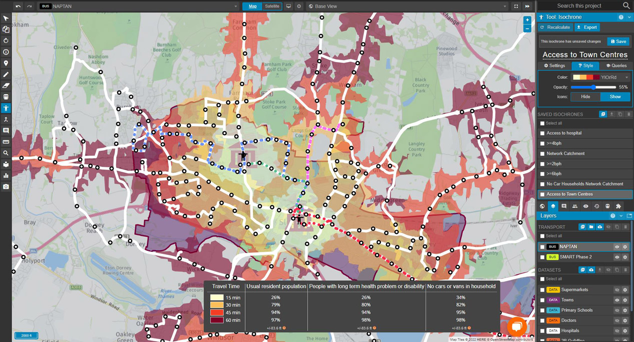
In the following tutorial, we will use the isochrone query tool to explore this in relation to rental developments in the Santa Clara area.
Exploring reach and travel time from a specific point
- Having constructed your transport network, import the dataset you wish to query, as per the instructions on datasets.
- Click
 to open the isochrone panel.
 - If you have selected
 you will be able to explore accessibility either
  or
or  a specific point on your map, at a time designated by the respective service day and departure/arrival time.
 - Click a point on your map to set it as either a start or destination point.
- Click
 on the QUERIES section of the isochrone tool panel to load the Isochrone Query editor.
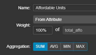
 - Having given our query a name, we're going to take a specific attribute from our dataset - in this case, total_affo, a number representing the amount of affordable units associated with that entity.
- Click OKAY and then
 to generate a list of affordable units within a range of travel times.
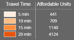
Constructing Queries
In constructing a query, you are required to specify several values:
- Name: This will be displayed on the travel time chart.
- Total per entity/From Attribute: Whether this query applies to each entity in a dataset, or to a specific attribute.
- Weight: A multiplier of either your total per entity or attribute value.
- Aggregation: Sum/average/minimum/maximum.
With each amendment to your query, you are required to click  on the isochrone tool panel before you can see your changes.
Filtering Dataset Entries
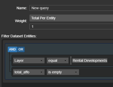
With dataset filtering, you can create complex filters using logical operations on the attributes of your data layers. Once you have added more than one rule with the  button, you can apply either an
 ![]() or
or ![]() boolean operator between them.
boolean operator between them.
Rules can also be nested in groups with the  button.
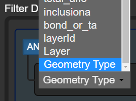
All dataset entries visible when filtering are derived from the dataset's attributes with the exception of Layer (which can be used to reference the entire layer by name) and Geometry Type.
You can read more about constructing queries and the available properties usable as filters here.
Filtering and Understanding Travel Time by Geometry Type
Below is an example of using the isochrone tool to quickly select all dataset features of a particular type (polygons, representing offices), and perform travel time analysis using them.
Further examples
You can find a range of examples of isochrone analysis that use queries to explore travel time and access time here.